The Cameron Peak Fire, Colorado, USA

It’s another ESIIL Earth Data Science Workflow
This notebook contains your next environmental data science (EDS) coding challenge! Before we get started, make sure to read or review the guidelines below. These will help make sure that your code is readable and reproducible.
Don’t get caught by these interactive coding notebook gotchas

Image source: https://alaskausfws.medium.com/whats-big-and-brown-and-loves-salmon-e1803579ee36
These are the most common issues that will keep you from getting started and delay your code review:
Run your code in the right environment to avoid import errors
We’ve created a coding environment for you to use that already has all the software and libraries you will need! When you try to run some code, you may be prompted to select a kernel. The kernel refers to the version of Python you are using. You should use the base kernel, which should be the default option.
Always run your code start to finish before submitting
Before you commit your work, make sure it runs reproducibly by clicking:
Restart(this button won’t appear until you’ve run some code), thenRun All
Check your code to make sure it’s clean and easy to read
Format all cells prior to submitting (right click on your code).
Use expressive names for variables so you or the reader knows what they are.
Use comments to explain your code – e.g.
# This is a comment, it starts with a hash sign
Label and describe your plots

Make sure each plot has:
- A title that explains where and when the data are from
- x- and y- axis labels with units where appropriate
- A legend where appropriate
The Cameron Peak Fire was the largest fire in Colorado history, with 326 square miles burned.
Observing vegetation health from space
We will look at the destruction and recovery of vegetation using NDVI (Normalized Difference Vegetation Index). How does it work? First, we need to learn about spectral reflectance signatures.
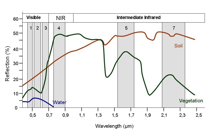
Every object reflects some wavelengths of light more or less than others. We can see this with our eyes, since, for example, plants reflect a lot of green in the summer, and then as that green diminishes in the fall they look more yellow or orange. The image below shows spectral signatures for water, soil, and vegetation:
 > Image source: SEOS
Project
> Image source: SEOS
Project
Healthy vegetation reflects a lot of Near-InfraRed (NIR) radiation. Dead ve Less healthy vegetation reflects a similar amounts of the visible light spectra, but less NIR radiation. We don’t see a huge drop in Green radiation until the plant is very stressed or dead. That means that NIR allows us to get ahead of what we can see with our eyes.
 > Image source: Spectral signature literature review by
px39n
> Image source: Spectral signature literature review by
px39n
Different species of plants reflect different spectral signatures, but the pattern of the signatures are similar. NDVI compares the amount of NIR reflectance to the amount of Red reflectance, thus accounting for many of the species differences and isolating the health of the plant. The formula for calculating NDVI is:
$$NDVI = \frac{(NIR - Red)}{(NIR + Red)}$$
Read more about NDVI and other vegetation indices: * earthdatascience.org * USGS
Import necessary libraries
In the cell below, making sure to keep the packages in order, add packages for:
- Working with DataFrames
- Working with GeoDataFrames
What are we using the rest of these packages for? See if you can figure it out as you complete the notebook.
# Install the development version of the earthpy package
!pip install git+https://github.com/earthlab/earthpy@apppears
Collecting git+https://github.com/earthlab/earthpy@apppears
  Cloning https://github.com/earthlab/earthpy (to revision apppears) to /tmp/pip-req-build-yoq146rv
  Running command git clone --filter=blob:none --quiet https://github.com/earthlab/earthpy /tmp/pip-req-build-yoq146rv
  Running command git checkout -b apppears --track origin/apppears
  Switched to a new branch 'apppears'
  Branch 'apppears' set up to track remote branch 'apppears' from 'origin'.
  Resolved https://github.com/earthlab/earthpy to commit 7241165d59af510d62bba312e48c7f513bc9dc05
  Installing build dependencies ... done
  Getting requirements to build wheel ... done
  Preparing metadata (pyproject.toml) ... done
Requirement already satisfied: geopandas in /opt/conda/lib/python3.11/site-packages (from earthpy==0.10.0) (0.14.2)
Requirement already satisfied: matplotlib>=2.0.0 in /opt/conda/lib/python3.11/site-packages (from earthpy==0.10.0) (3.8.4)
Requirement already satisfied: numpy>=1.14.0 in /opt/conda/lib/python3.11/site-packages (from earthpy==0.10.0) (1.24.3)
Requirement already satisfied: rasterio in /opt/conda/lib/python3.11/site-packages (from earthpy==0.10.0) (1.3.9)
Requirement already satisfied: scikit-image in /opt/conda/lib/python3.11/site-packages (from earthpy==0.10.0) (0.22.0)
Requirement already satisfied: requests in /opt/conda/lib/python3.11/site-packages (from earthpy==0.10.0) (2.31.0)
Requirement already satisfied: keyring in /opt/conda/lib/python3.11/site-packages (from earthpy==0.10.0) (25.1.0)
Requirement already satisfied: contourpy>=1.0.1 in /opt/conda/lib/python3.11/site-packages (from matplotlib>=2.0.0->earthpy==0.10.0) (1.2.0)
Requirement already satisfied: cycler>=0.10 in /opt/conda/lib/python3.11/site-packages (from matplotlib>=2.0.0->earthpy==0.10.0) (0.11.0)
Requirement already satisfied: fonttools>=4.22.0 in /opt/conda/lib/python3.11/site-packages (from matplotlib>=2.0.0->earthpy==0.10.0) (4.51.0)
Requirement already satisfied: kiwisolver>=1.3.1 in /opt/conda/lib/python3.11/site-packages (from matplotlib>=2.0.0->earthpy==0.10.0) (1.4.4)
Requirement already satisfied: packaging>=20.0 in /opt/conda/lib/python3.11/site-packages (from matplotlib>=2.0.0->earthpy==0.10.0) (24.0)
Requirement already satisfied: pillow>=8 in /opt/conda/lib/python3.11/site-packages (from matplotlib>=2.0.0->earthpy==0.10.0) (10.3.0)
Requirement already satisfied: pyparsing>=2.3.1 in /opt/conda/lib/python3.11/site-packages (from matplotlib>=2.0.0->earthpy==0.10.0) (3.0.9)
Requirement already satisfied: python-dateutil>=2.7 in /opt/conda/lib/python3.11/site-packages (from matplotlib>=2.0.0->earthpy==0.10.0) (2.9.0)
Requirement already satisfied: fiona>=1.8.21 in /opt/conda/lib/python3.11/site-packages (from geopandas->earthpy==0.10.0) (1.9.6)
Requirement already satisfied: pandas>=1.4.0 in /opt/conda/lib/python3.11/site-packages (from geopandas->earthpy==0.10.0) (2.2.1)
Requirement already satisfied: pyproj>=3.3.0 in /opt/conda/lib/python3.11/site-packages (from geopandas->earthpy==0.10.0) (3.6.1)
Requirement already satisfied: shapely>=1.8.0 in /opt/conda/lib/python3.11/site-packages (from geopandas->earthpy==0.10.0) (2.0.4)
Requirement already satisfied: jaraco.classes in /opt/conda/lib/python3.11/site-packages (from keyring->earthpy==0.10.0) (3.4.0)
Requirement already satisfied: jaraco.functools in /opt/conda/lib/python3.11/site-packages (from keyring->earthpy==0.10.0) (4.0.1)
Requirement already satisfied: jaraco.context in /opt/conda/lib/python3.11/site-packages (from keyring->earthpy==0.10.0) (5.3.0)
Requirement already satisfied: importlib-metadata>=4.11.4 in /opt/conda/lib/python3.11/site-packages (from keyring->earthpy==0.10.0) (7.1.0)
Requirement already satisfied: SecretStorage>=3.2 in /opt/conda/lib/python3.11/site-packages (from keyring->earthpy==0.10.0) (3.3.3)
Requirement already satisfied: jeepney>=0.4.2 in /opt/conda/lib/python3.11/site-packages (from keyring->earthpy==0.10.0) (0.8.0)
Requirement already satisfied: affine in /opt/conda/lib/python3.11/site-packages (from rasterio->earthpy==0.10.0) (2.3.0)
Requirement already satisfied: attrs in /opt/conda/lib/python3.11/site-packages (from rasterio->earthpy==0.10.0) (23.2.0)
Requirement already satisfied: certifi in /opt/conda/lib/python3.11/site-packages (from rasterio->earthpy==0.10.0) (2024.2.2)
Requirement already satisfied: click>=4.0 in /opt/conda/lib/python3.11/site-packages (from rasterio->earthpy==0.10.0) (8.1.7)
Requirement already satisfied: cligj>=0.5 in /opt/conda/lib/python3.11/site-packages (from rasterio->earthpy==0.10.0) (0.7.2)
Requirement already satisfied: snuggs>=1.4.1 in /opt/conda/lib/python3.11/site-packages (from rasterio->earthpy==0.10.0) (1.4.7)
Requirement already satisfied: click-plugins in /opt/conda/lib/python3.11/site-packages (from rasterio->earthpy==0.10.0) (1.1.1)
Requirement already satisfied: setuptools in /opt/conda/lib/python3.11/site-packages (from rasterio->earthpy==0.10.0) (69.5.1)
Requirement already satisfied: charset-normalizer<4,>=2 in /opt/conda/lib/python3.11/site-packages (from requests->earthpy==0.10.0) (3.3.2)
Requirement already satisfied: idna<4,>=2.5 in /opt/conda/lib/python3.11/site-packages (from requests->earthpy==0.10.0) (3.7)
Requirement already satisfied: urllib3<3,>=1.21.1 in /opt/conda/lib/python3.11/site-packages (from requests->earthpy==0.10.0) (2.2.1)
Requirement already satisfied: scipy>=1.8 in /opt/conda/lib/python3.11/site-packages (from scikit-image->earthpy==0.10.0) (1.12.0)
Requirement already satisfied: networkx>=2.8 in /opt/conda/lib/python3.11/site-packages (from scikit-image->earthpy==0.10.0) (3.1)
Requirement already satisfied: imageio>=2.27 in /opt/conda/lib/python3.11/site-packages (from scikit-image->earthpy==0.10.0) (2.33.1)
Requirement already satisfied: tifffile>=2022.8.12 in /opt/conda/lib/python3.11/site-packages (from scikit-image->earthpy==0.10.0) (2023.4.12)
Requirement already satisfied: lazy_loader>=0.3 in /opt/conda/lib/python3.11/site-packages (from scikit-image->earthpy==0.10.0) (0.3)
Requirement already satisfied: six in /opt/conda/lib/python3.11/site-packages (from fiona>=1.8.21->geopandas->earthpy==0.10.0) (1.16.0)
Requirement already satisfied: zipp>=0.5 in /opt/conda/lib/python3.11/site-packages (from importlib-metadata>=4.11.4->keyring->earthpy==0.10.0) (3.17.0)
Requirement already satisfied: pytz>=2020.1 in /opt/conda/lib/python3.11/site-packages (from pandas>=1.4.0->geopandas->earthpy==0.10.0) (2024.1)
Requirement already satisfied: tzdata>=2022.7 in /opt/conda/lib/python3.11/site-packages (from pandas>=1.4.0->geopandas->earthpy==0.10.0) (2023.3)
Requirement already satisfied: cryptography>=2.0 in /opt/conda/lib/python3.11/site-packages (from SecretStorage>=3.2->keyring->earthpy==0.10.0) (42.0.5)
Requirement already satisfied: more-itertools in /opt/conda/lib/python3.11/site-packages (from jaraco.classes->keyring->earthpy==0.10.0) (10.2.0)
Requirement already satisfied: backports.tarfile in /opt/conda/lib/python3.11/site-packages (from jaraco.context->keyring->earthpy==0.10.0) (1.1.1)
Requirement already satisfied: cffi>=1.12 in /opt/conda/lib/python3.11/site-packages (from cryptography>=2.0->SecretStorage>=3.2->keyring->earthpy==0.10.0) (1.16.0)
Requirement already satisfied: pycparser in /opt/conda/lib/python3.11/site-packages (from cffi>=1.12->cryptography>=2.0->SecretStorage>=3.2->keyring->earthpy==0.10.0) (2.22)
import getpass
import json
import os
import pathlib
from glob import glob

import earthpy.appeears as eaapp
import geopandas as gpd
import hvplot.pandas
import hvplot.xarray
import pandas as pd
import rioxarray as rxr
import xarray as xr
We have one more setup task. We’re not going to be able to load all our data directly from the web to Python this time. That means we need to set up a place for it.
GOTCHA ALERT
A lot of times in Python we say “directory” to mean a “folder” on your computer. The two words mean the same thing in this context.
Your task
In the cell below, replace ‘my-data-folder’ with a descriptive directory name.
data_dir = os.path.join(
    pathlib.Path.home(), 'cameron-peak')
# Make the data directory
os.makedirs(data_dir, exist_ok=True)
Study Area: Cameron Peak Fire Boundary
Earth Data Science data formats
In Earth Data Science, we get data in three main formats:
| Data type | Descriptions | Common file formats | Python type |
|---|---|---|---|
| Time Series | The same data points (e.g. streamflow) collected multiple times over time | Tabular formats (e.g. .csv, or .xlsx) | pandas DataFrame |
| Vector | Points, lines, and areas (with coordinates) | Shapefile (often an archive like a .zip file because a Shapefile is actually a collection of at least 3 files) |
geopandas GeoDataFrame |
| Raster | Evenly spaced spatial grid (with coordinates) | GeoTIFF (.tif), NetCDF (.nc), HDF (.hdf) |
rioxarray DataArray |
Read more
Check out the sections about about vector data and raster data in the textbook.
What do you think?
For this coding challenge, we are interested in the boundary of the Cameron Peak Fire. In the cell below, answer the following question: What data type do you think the reservation boundaries will be?
Your task:
- Search the National Interagency Fire Center Wildfire Boundary catalog for and incident name “Cameron Peak”
- Copy the API results to your clipboard.
- Load the data into Python using the
geopandaslibrary, e.g.:python gpd.read_file(url)- Call your data at the end of the cell for testing.
# Download the Cameron Peak fire boundary

url = (
    "https://services3.arcgis.com/T4QMspbfLg3qTGWY/arcgis/rest/services"
    "/WFIGS_Interagency_Perimeters/FeatureServer/0/query"
    "?where=poly_IncidentName%20%3D%20'CAMERON%20PEAK'"
    "&outFields=*&outSR=4326&f=json")

gdf = gpd.read_file(url)
gdf
/opt/conda/lib/python3.11/site-packages/geopandas/io/file.py:399: FutureWarning: errors='ignore' is deprecated and will raise in a future version. Use to_datetime without passing `errors` and catch exceptions explicitly instead
  as_dt = pd.to_datetime(df[k], errors="ignore")
/opt/conda/lib/python3.11/site-packages/geopandas/io/file.py:399: FutureWarning: errors='ignore' is deprecated and will raise in a future version. Use to_datetime without passing `errors` and catch exceptions explicitly instead
  as_dt = pd.to_datetime(df[k], errors="ignore")
/opt/conda/lib/python3.11/site-packages/geopandas/io/file.py:399: FutureWarning: errors='ignore' is deprecated and will raise in a future version. Use to_datetime without passing `errors` and catch exceptions explicitly instead
  as_dt = pd.to_datetime(df[k], errors="ignore")
/opt/conda/lib/python3.11/site-packages/geopandas/io/file.py:399: FutureWarning: errors='ignore' is deprecated and will raise in a future version. Use to_datetime without passing `errors` and catch exceptions explicitly instead
  as_dt = pd.to_datetime(df[k], errors="ignore")
/opt/conda/lib/python3.11/site-packages/geopandas/io/file.py:399: FutureWarning: errors='ignore' is deprecated and will raise in a future version. Use to_datetime without passing `errors` and catch exceptions explicitly instead
  as_dt = pd.to_datetime(df[k], errors="ignore")
/opt/conda/lib/python3.11/site-packages/geopandas/io/file.py:399: FutureWarning: errors='ignore' is deprecated and will raise in a future version. Use to_datetime without passing `errors` and catch exceptions explicitly instead
  as_dt = pd.to_datetime(df[k], errors="ignore")
/opt/conda/lib/python3.11/site-packages/geopandas/io/file.py:399: FutureWarning: errors='ignore' is deprecated and will raise in a future version. Use to_datetime without passing `errors` and catch exceptions explicitly instead
  as_dt = pd.to_datetime(df[k], errors="ignore")
/opt/conda/lib/python3.11/site-packages/geopandas/io/file.py:399: FutureWarning: errors='ignore' is deprecated and will raise in a future version. Use to_datetime without passing `errors` and catch exceptions explicitly instead
  as_dt = pd.to_datetime(df[k], errors="ignore")
/opt/conda/lib/python3.11/site-packages/geopandas/io/file.py:399: FutureWarning: errors='ignore' is deprecated and will raise in a future version. Use to_datetime without passing `errors` and catch exceptions explicitly instead
  as_dt = pd.to_datetime(df[k], errors="ignore")
/opt/conda/lib/python3.11/site-packages/geopandas/io/file.py:399: FutureWarning: errors='ignore' is deprecated and will raise in a future version. Use to_datetime without passing `errors` and catch exceptions explicitly instead
  as_dt = pd.to_datetime(df[k], errors="ignore")
/opt/conda/lib/python3.11/site-packages/geopandas/io/file.py:399: FutureWarning: errors='ignore' is deprecated and will raise in a future version. Use to_datetime without passing `errors` and catch exceptions explicitly instead
  as_dt = pd.to_datetime(df[k], errors="ignore")
/opt/conda/lib/python3.11/site-packages/geopandas/io/file.py:399: FutureWarning: errors='ignore' is deprecated and will raise in a future version. Use to_datetime without passing `errors` and catch exceptions explicitly instead
  as_dt = pd.to_datetime(df[k], errors="ignore")
/opt/conda/lib/python3.11/site-packages/geopandas/io/file.py:399: FutureWarning: errors='ignore' is deprecated and will raise in a future version. Use to_datetime without passing `errors` and catch exceptions explicitly instead
  as_dt = pd.to_datetime(df[k], errors="ignore")
/opt/conda/lib/python3.11/site-packages/geopandas/io/file.py:399: FutureWarning: errors='ignore' is deprecated and will raise in a future version. Use to_datetime without passing `errors` and catch exceptions explicitly instead
  as_dt = pd.to_datetime(df[k], errors="ignore")
/opt/conda/lib/python3.11/site-packages/geopandas/io/file.py:399: FutureWarning: errors='ignore' is deprecated and will raise in a future version. Use to_datetime without passing `errors` and catch exceptions explicitly instead
  as_dt = pd.to_datetime(df[k], errors="ignore")
| OBJECTID | poly_SourceOID | poly_IncidentName | poly_FeatureCategory | poly_MapMethod | poly_GISAcres | poly_CreateDate | poly_DateCurrent | poly_PolygonDateTime | poly_IRWINID | ... | attr_Source | attr_IsCpxChild | attr_CpxName | attr_CpxID | attr_SourceGlobalID | GlobalID | Shape__Area | Shape__Length | attr_IncidentComplexityLevel | geometry | |
|---|---|---|---|---|---|---|---|---|---|---|---|---|---|---|---|---|---|---|---|---|---|
| 0 | 14659 | 10393 | Cameron Peak | Wildfire Final Fire Perimeter | Infrared Image | 208913.3 | NaT | 2023-03-14 15:13:42.810000+00:00 | 2020-10-06 21:30:00+00:00 | {53741A13-D269-4CD5-AF91-02E094B944DA} | ... | FODR | None | None | None | {5F5EC9BA-5F85-495B-8B97-1E0969A1434E} | e8e4ffd4-db84-4d47-bd32-d4b0a8381fff | 0.089957 | 5.541765 | None | MULTIPOLYGON (((-105.88333 40.54598, -105.8837... |
1 rows × 115 columns
ans_gdf = _
gdf_pts = 0

if isinstance(ans_gdf, gpd.GeoDataFrame):
    print('\u2705 Great work! You downloaded and opened a GeoDataFrame')
    gdf_pts +=2
else:
    print('\u274C Hmm, your answer is not a GeoDataFrame')

print('\u27A1 You earned {} of 2 points for downloading data'.format(gdf_pts))
✅ Great work! You downloaded and opened a GeoDataFrame
➡ You earned 2 of 2 points for downloading data
Site Map
We always want to create a site map when working with geospatial data. This helps us see that we’re looking at the right location, and learn something about the context of the analysis.
Your task
- Plot your Cameron Peak Fire shapefile on an interactive map
- Make sure to add a title
- Add ESRI World Imagery as the basemap/background using the
tiles=...parameter
# Plot the Cameron Peak Fire boundary
gdf.hvplot(
    title='Cameron Peak Fire, 2020',
    tiles='EsriImagery')
Exploring the AppEEARS API for NASA Earthdata access
Over the next four cells, you will download MODIS NDVI data for the study period. MODIS is a multispectral instrument that measures Red and NIR data (and so can be used for NDVI). There are two MODIS sensors on two different platforms: satellites Terra and Aqua.
Read more
Learn more about MODIS datasets and the science they support
Since we’re asking for a special download that only covers our study
area, we can’t just find a link to the data - we have to negotiate with
the data server. We’re doing this using the
APPEEARS API
(Application Programming Interface). The API makes it possible for you
to request data using code. You can use code from the earthpy library
to handle the API request.
Your task
Often when we want to do something more complex in coding we find an example and modify it. This download code is already almost a working example. Your task will be:
- Enter your NASA Earthdata username and password when prompted
- Replace the start and end dates in the task parameters. Download data from July, when greenery is at its peak in the Northern Hemisphere.
- Replace the year range. You should get 3 years before and after the fire so you can see the change!
- Replace
gdfwith the name of your site geodataframe.What would the product and layer name be if you were trying to download Landsat Surface Temperature Analysis Ready Data (ARD) instead of MODIS NDVI?
# Initialize AppeearsDownloader for MODIS NDVI data
ndvi_downloader = eaapp.AppeearsDownloader(
    download_key='cp-ndvi',
    ea_dir=data_dir,
    product='MOD13Q1.061',
    layer='_250m_16_days_NDVI',
    start_date="01-01",
    end_date="01-31",
    recurring=True,
    year_range=[2021, 2021],
    polygon=gdf
)
# Initialize AppeearsDownloader for MODIS NDVI data
ndvi_downloader = eaapp.AppeearsDownloader(
    download_key='cp-ndvi',
    ea_dir=data_dir,
    product='MOD13Q1.061',
    layer='_250m_16_days_NDVI',
    start_date="07-01",
    end_date="07-31",
    recurring=True,
    year_range=[2018, 2023],
    polygon=gdf
)
ndvi_downloader.download_files(cache=True)
Putting it together: Working with multi-file raster datasets in Python
Now you need to load all the downloaded files into Python. Let’s start by getting all the file names. You will also need to extract the date from the filename. Check out the lesson on getting information from filenames in the textbook.
GOTCHA ALERT
globdoesn’t necessarily find files in the order you would expect. Make sure to sort your file names like it says in the textbook.
# Get a list of NDVI tif file paths

ndvi_paths = sorted(glob(os.path.join(data_dir, 'cp-ndvi', '*', '*NDVI*.tif')))
len(ndvi_paths)
ndvi_paths
['/home/jovyan/cameron-peak/cp-ndvi/MOD13Q1.061_2018167_to_2023212/MOD13Q1.061__250m_16_days_NDVI_doy2018177_aid0001.tif',
 '/home/jovyan/cameron-peak/cp-ndvi/MOD13Q1.061_2018167_to_2023212/MOD13Q1.061__250m_16_days_NDVI_doy2018193_aid0001.tif',
 '/home/jovyan/cameron-peak/cp-ndvi/MOD13Q1.061_2018167_to_2023212/MOD13Q1.061__250m_16_days_NDVI_doy2018209_aid0001.tif',
 '/home/jovyan/cameron-peak/cp-ndvi/MOD13Q1.061_2018167_to_2023212/MOD13Q1.061__250m_16_days_NDVI_doy2019177_aid0001.tif',
 '/home/jovyan/cameron-peak/cp-ndvi/MOD13Q1.061_2018167_to_2023212/MOD13Q1.061__250m_16_days_NDVI_doy2019193_aid0001.tif',
 '/home/jovyan/cameron-peak/cp-ndvi/MOD13Q1.061_2018167_to_2023212/MOD13Q1.061__250m_16_days_NDVI_doy2019209_aid0001.tif',
 '/home/jovyan/cameron-peak/cp-ndvi/MOD13Q1.061_2018167_to_2023212/MOD13Q1.061__250m_16_days_NDVI_doy2020177_aid0001.tif',
 '/home/jovyan/cameron-peak/cp-ndvi/MOD13Q1.061_2018167_to_2023212/MOD13Q1.061__250m_16_days_NDVI_doy2020193_aid0001.tif',
 '/home/jovyan/cameron-peak/cp-ndvi/MOD13Q1.061_2018167_to_2023212/MOD13Q1.061__250m_16_days_NDVI_doy2020209_aid0001.tif',
 '/home/jovyan/cameron-peak/cp-ndvi/MOD13Q1.061_2018167_to_2023212/MOD13Q1.061__250m_16_days_NDVI_doy2021177_aid0001.tif',
 '/home/jovyan/cameron-peak/cp-ndvi/MOD13Q1.061_2018167_to_2023212/MOD13Q1.061__250m_16_days_NDVI_doy2021193_aid0001.tif',
 '/home/jovyan/cameron-peak/cp-ndvi/MOD13Q1.061_2018167_to_2023212/MOD13Q1.061__250m_16_days_NDVI_doy2021209_aid0001.tif',
 '/home/jovyan/cameron-peak/cp-ndvi/MOD13Q1.061_2018167_to_2023212/MOD13Q1.061__250m_16_days_NDVI_doy2022177_aid0001.tif',
 '/home/jovyan/cameron-peak/cp-ndvi/MOD13Q1.061_2018167_to_2023212/MOD13Q1.061__250m_16_days_NDVI_doy2022193_aid0001.tif',
 '/home/jovyan/cameron-peak/cp-ndvi/MOD13Q1.061_2018167_to_2023212/MOD13Q1.061__250m_16_days_NDVI_doy2022209_aid0001.tif',
 '/home/jovyan/cameron-peak/cp-ndvi/MOD13Q1.061_2018167_to_2023212/MOD13Q1.061__250m_16_days_NDVI_doy2023177_aid0001.tif',
 '/home/jovyan/cameron-peak/cp-ndvi/MOD13Q1.061_2018167_to_2023212/MOD13Q1.061__250m_16_days_NDVI_doy2023193_aid0001.tif',
 '/home/jovyan/cameron-peak/cp-ndvi/MOD13Q1.061_2018167_to_2023212/MOD13Q1.061__250m_16_days_NDVI_doy2023209_aid0001.tif']
Repeating tasks in Python
Now you should have a few dozen files! For each file, you need to:
- Load the file in using the
rioxarraylibrary - Get the date from the file name
- Add the date as a dimension coordinate
- Give your data variable a name
- Divide by the scale factor of 10000
You don’t want to write out the code for each file! That’s a recipe for
copy pasta. Luckily, Python has tools for doing similar tasks
repeatedly. In this case, you’ll use one called a for loop.
There’s some code below that uses a for loop in what is called an
accumulation pattern to process each file. That means that you will
save the results of your processing to a list each time you process the
files, and then merge all the arrays in the list.
Your task
- Look at the file names. How many characters from the end is the date?
- Replace any required variable names with your chosen variable names
- Change the
scale_factorvariable to be the correct scale factor for this NDVI dataset (HINT: NDVI should range between 0 and 1)- Using indices or regular
scale_factor = 10000
doy_start = -19
doy_end = -12
ndvi_das = []
for ndvi_path in ndvi_paths:
    # Get date from file name
    doy = ndvi_path[doy_start:doy_end]
    date = pd.to_datetime(doy, format='%Y%j')

    # Open dataset
    da = rxr.open_rasterio(ndvi_path, masked=True).squeeze()

    # Add date dimension and clean up metadata
    da = da.assign_coords({'date': date})
    da = da.expand_dims({'date': 1})
    da.name = 'NDVI'

    # Multiple by scale factor
    da = da / scale_factor

    # Prepare for concatenation
    ndvi_das.append(da)

len(ndvi_das)
18
Next, stack your arrays by date into a time series using the
xr.combine_by_coords() function. You will have to tell it which
dimension you want to stack your data in.
Plot the change in NDVI spatially
Complete the following: * Select data from 2021 to 2023 (3 years after the fire) * Take the temporal mean (over the date, not spatially) * Get the NDVI variable (should be a DataArray, not a Dataset) * Repeat for the data from 2018 to 2020 (3 years before the fire) * Subtract the 2018-2020 time period from the 2021-2023 time period * Plot the result using a diverging color map like
cmap=plt.cm.PiYGThere are different types of color maps for different types of data. In this case, we want decreases to be a different color from increases, so we should use a diverging color map. Check out available colormaps in the matplotlib documentation.
For an extra challenge, add the fire boundary to the plot
ndvi_da = xr.combine_by_coords(ndvi_das, coords=['date'])
ndvi_da
<xarray.Dataset>
Dimensions:      (x: 339, y: 153, date: 18)
Coordinates:
    band         int64 1
  * x            (x) float64 -105.9 -105.9 -105.9 ... -105.2 -105.2 -105.2
  * y            (y) float64 40.78 40.78 40.77 40.77 ... 40.47 40.47 40.46 40.46
    spatial_ref  int64 0
  * date         (date) datetime64[ns] 2018-06-26 2018-07-12 ... 2023-07-28
Data variables:
NDVI (date, y, x) float32 0.5672 0.5711 0.6027 ... 0.6327 0.6327# Compute the difference in NDVI before and after the fire
# Plot the difference
ndvi_diff = (
ndvi_da
.sel(date=slice('2021', '2023'))
.mean('date')
.NDVI
- ndvi_da
.sel(date=slice('2018', '2020'))
.mean('date')
.NDVI
)
(
ndvi_diff.hvplot(x='x', y='y', cmap='PiYG', geo=True)
*
gdf.hvplot(geo=True, fill_color=None, line_color='black')
)
Is the NDVI lower within the fire boundary after the fire?
You will compute the mean NDVI inside and outside the fire boundary.
First, use the code below to get a GeoDataFrame of the area outside
the Reservation. Your task: * Check the variable names - Make sure that
the code uses your boundary GeoDataFrame * How could you test if the
geometry was modified correctly? Add some code to take a look at the
results.
out_gdf = (
    gpd.GeoDataFrame(geometry=gdf.envelope)
    .overlay(gdf, how='difference'))
Next, clip your DataArray to the boundaries for both inside and outside
the reservation. You will need to replace the GeoDataFrame name with
your own. Check out the lesson on clipping data with the rioxarray
library in the
textbook.
GOTCHA ALERT
It’s important to use
from_disk=Truewhen clipping large arrays like this. It allows the computer to use less valuable memory resources when clipping - you will probably find that otherwise the cell below crashes the kernel
# Clip data to both inside and outside the boundary

ndvi_cp_da = ndvi_da.rio.clip(gdf.geometry, from_disk=True)
ndvi_out_da = ndvi_da.rio.clip(out_gdf.geometry, from_disk=True)
Your Task
For both inside and outside the fire boundary:
- Group the data by year
- Take the mean. You always need to tell reducing methods in
xarraywhat dimensions you want to reduce. When you want to summarize data across all dimensions, you can use the...syntax, e.g..mean(...)as a shorthand.- Select the NDVI variable
- Convert to a DataFrame using the
to_dataframe()method- Join the two DataFrames for plotting using the
.join()method. You will need to rename the columns using thelsuffix=andrsuffix=parameters
GOTCHA ALERT
The DateIndex in pandas is a little different from the Datetime Dimension in xarray. You will need to use the
.dt.yearsyntax to access information about the year, not just.year.
Finally, plot annual July means for both inside and outside the Reservation on the same plot.
:::
# Compute mean annual July NDVI

jul_ndvi_cp_df = (
    ndvi_cp_da
    .groupby(ndvi_cp_da.date.dt.year)
    .mean(...)
    .NDVI.to_dataframe())
jul_ndvi_out_df = (
    ndvi_out_da
    .groupby(ndvi_out_da.date.dt.year)
    .mean(...)
    .NDVI.to_dataframe())

# Plot inside and outside the reservation
jul_ndvi_df = (
    jul_ndvi_cp_df[['NDVI']]
    .join(
        jul_ndvi_out_df[['NDVI']],
        lsuffix=' Burned Area', rsuffix=' Unburned Area')
)

jul_ndvi_df.hvplot(
    title='NDVI before and after the Cameron Peak Fire'
)
Now, take the difference between outside and inside the Reservation and plot that. What do you observe? Don’t forget to write a headline and description of your plot!
# Plot difference inside and outside the reservation

jul_ndvi_df['difference'] = (
    jul_ndvi_df['NDVI Burned Area']
    - jul_ndvi_df['NDVI Unburned Area'])
jul_ndvi_df.difference.hvplot(
    title='Difference between NDVI within and outside the Cameron Peak Fire'
)
Your turn! Repeat this workflow in a different time and place.
It’s not just fires that affect NDVI! You could look at:
- Recovery after a national disaster, like a wildfire or hurricane
- Drought
- Deforestation
- Irrigation
- Beaver reintroduction
%%capture
%%bash
jupyter nbconvert *.ipynb --to html